[Paper Review] VQ-VAE: Vector Quantised-Variational AutoEncoder
VQ-VAE는 VAE와 discrete latent representation을 결합한 모델입니다. 기존 VAE의 continuous latent representation에서 각 vector를 codebook의 entry 중 가장 가까운 vector로 치환함으로써 discrete하게 변환하는 것인데요. 이 과정이 바로 Vector Quantisation(VQ)입니다. 이렇게 하면 continuous representation을 학습하는 VAE 모델과 비슷한 성능을 보이면서 discrete distribution의 유연성도 취할 수 있다는 장점이 있습니다. VQ-VAE에 대해 자세히 알아 보기에 앞서, VAE와의 차이점을 정리해보면 다음과 같습니다.
| VAE | VQ-VAE | |
|---|---|---|
| encoder output | continuous representation | discrete representation |
| prior $p(z)$ | 고정 (가우시안 분포로 가정) | 학습 |
1. 모델 구조
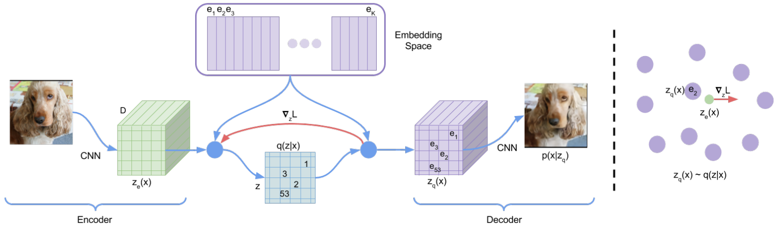 VQ-VAE architecture
1. Discrete Latent variables
VQ-VAE와 VAE의 가장 큰 차이점은 continuous representation이 아니라 discrete representation을 학습한다는 점에 있습니다. 논문에 따르면, continuous representation보다 discrete representation이 언어, 음성, 이미지 등 서로 다른 유형이나 형식의 데이터(modality)에서 자연스러운 표현 방법일 수 있다고 합니다. 언어는 본질적으로 불연속적이고, 음성도 기호들의 sequence로 표현되며, 이미지는 언어로 간결하게 설명할 수 있기 때문입니다.
latent embedding space $e \in R^{K \times D}$
- $K$는 discrete latent space의 크기 $e_i \in R^D, i \in 1, 2, … K$
- $D$는 각각의 latent embedding vector $e_i$의 차원 크기
2. Learning
2.1 Forward Computation
Step 1encoder는 input 이미지 $x$를 입력받아서 continuous representation $z_e(x)$를 출력합니다.Step 2continuous representation $z_e(x)$는 Vector Quantization를 통해 embedding space $e$에서 가장 가까운 embedding vector $z_q(x)$로 매핑됩니다. $z_q(x)$가 사전에 정의된 codebook vector 중 가장 가까운 vector로 변환되는 것입니다. codebook은 encoder와 decoder가 공유하는 lookup table 같은 개념입니다.
Step 3decoder는 $z_q(x)$를 입력받아서 input 이미지 $x$를 복원합니다.
2.2 Backward Computation
Step 1loss function $L$의 gradient $\bigtriangledown_zL$는 decoder input $z_q(x)$에 대해 계산됩니다.Step 2gradient $\bigtriangledown_zL$는 그대로 복사되어 encoder output $z_e(x)$에 전달됩니다. Vector Quantization 과정이 불연속적이어서 직접적인 gradient 계산이 불가능하기 때문에 이러한 방식을 사용합니다. encoder의 output representation과 decoder의 input이 동일한 $D$ 차원의 space를 공유하고 있기 때문에, gradients는 reconstruction error를 낮추기 위해 encoder가 output representation를 어떻게 변화시켜야 하는지에 대한 유용한 정보를 포함하고 있습니다. 즉, encoder는 gradient 정보를 사용하여 input 이미지를 더 잘 표현할 수 있도록 학습합니다.
2.3 loss function
\[L = \log p(x | z_q(x)) + \| \text{sg}[z_e(x)] - e \|^2_2 + \beta \| z_e(x) - \text{sg}[e] \|^2_2\]- 첫번째 항은 reconstruction error입니다.
- 두번째 항은 embedding vector $e_i$를 encoder output $z_e(x)$로 이동시키기 위한 $l_2$ error로, code book을 업데이트하는 데에만 사용됩니다.
- 세번째 항은 commitment loss입니다.
- decoder는 첫번째 항에서, encoder는 첫번째 항과 세번째 항에서, embedding은 두번째 항에서 최적화됩니다.
- sg는 stop-gradient로, 각자 자기 영역만 업데이트하게 해서 gradient 흐름이 꼬이지 않도록 합니다.
3. Prior
VQ-VAE의 학습 자체는 prior 없이 이루어집니다. 그리고 decoder에 latent를 입력해 이미지를 단순히 reconstruction하는 데에는 prior가 필요하지 않습니다. VQ-VAE의 학습이 끝난 뒤에 생성 모델로 사용할 때는 아래와 같은 과정을 거치게 됩니다.
Step 1latent variable $z$를 prior로부터 sampling합니다.Step 2sampling한 latent index들을 codebook vector로 변환(VQ)합니다.Step 3decoder에 입력해 $\hat{x}$ 생성합니다.
위 과정에서 필요한 prior를 학습하는 과정은 아래와 같습니다.
Step 1모든 학습 이미지를 Encoder에 통과시킵니다.Step 2Vector Quantization을 거쳐 latent map을 얻습니다. codebook의 사이즈 $K$가 512라면, latent map은 0에서 511 사이의 index 값들로 이루어진 행렬입니다.Step 3Step 2에서 얻은 latent map들로 prior를 학습합니다. 이미 학습된 VQ-VAE는 고정합니다.
이 때 discrete latent representation과 autoregressive prior를 결합해서 discrete하고 유용한 latent variable을 학습함으로써 고품질의 데이터를 생성하는 것이 VQ-VAE의 가장 큰 특징입니다. autoregressive prior는 모델이 latent variable $z$를 생성할 때 이전의 변수를 기반으로 다음 변수를 생성하는 방식입니다. 즉, input은 이전까지의 latent index들이고 target은 다음 latent index로 데이터셋을 구성해서 학습하는 것입니다. 이는 latent variable $z$들이 sequence 형태로 존재하며, 각 variable은 이전 variable에 의존하여 결정되는 분포를 따른다는 것을 의미합니다.
저자들은 PixelCNN과 WaveNet을 각각 이미지와 오디오 데이터에 대한 autoregressive prior로 사용했습니다. PixelCNN은 $x_i$가 하나의 픽셀일 때, 이미지 $x$에 대한 픽셀들의 joint distribution $p(x)$는 conditional distribution의 곱으로 모델링합니다. 이미지의 각 픽셀이 이전 픽셀들에 의존하는 방식으로 이미지를 생성하는 것입니다. 마찬가지로 WaveNet은 음성 신호의 각 샘플을 이전 샘플에 의존하여 생성합니다.
\[p(x)= \prod_{i=1}^{n^2}p(x_i \vert x_1, …, x_{i-1})\]![]() PixelCNN architecture
PixelCNN architecture
2. 모델 학습
기본적인 VAE 구조를 사용해서 CIFAR10 데이터셋을 학습시켰습니다.
Encoder- 2개의 convolutional layer (stride 2, window size 4 X 4)
- 2개의 residual 3 X 3 block
Decoder- 2개의 residual 3 X 3 block
- 2개의 transposed convolutional layer (stride 2, window size 4 X 4)
- hidden unit 256개
- ADAM optimiser
- Learning rate 2e-4
- batch size 128